Totally Accessible MRI
Dr. Lipton has presented his one-week intensive course, “Totally Accessible MRI” since 2001. Currently, the course is given live at Columbia University Irving Medical Center in New York City twice annually and receives consistently outstanding reviews. Taking students through MRI “from A to Z” without assuming any specific technical or mathematical background, “Totally Accessible MRI” comprises 30 hours of highly interactive instruction. Two key features underpinning the accessibility of the course are its rigorous yet largely non-mathematical approach and its emphasis on direct relevance of key concepts to the creation of clinically useful MR images of all types.
Your course is super interesting and clear for people like me who are not too physics/mathematics inclined.
I wish you a Happy Teacher’s Day… I’m lucky that I found those videos and a great teacher like you. Thank you with lots of love from India
I just wanted to drop you a line to say that I’m around half way through your internet series of lectures and they are fabulous. I work in radiotherapy, as a physicist, and although I had a vague grasp of the principles of NMR, your lecture series has clarified so many confusions for me. I also really appreciate your teaching style and hope I can learn a little of that too!
Thank you for this wonderful collection of lectures on MRI, Dr. Lipton!
This man is a rockstar!
Your engaging, logically structured, and clear teaching style really made all the difference for me. The way you explained complex concepts like quantum mechanics in a simple and approachable way helped me build a solid foundation, and I look forward to building on this knowledge.
The content of the course is remarkable and your teaching skills are also incredible.
GREAT WORK… GREAT TEACHING…HATS OFF TO YOU SIR…
Absolutely fantastic! So far, best tutorial for MRI physics I’ve ever encountered. I’ve binge watched in the past few days and I’m excited about the next chapters.
I just started this wonderful lecture. Thank you!
Thank you so much for recording these lecture and posting them!! NOTHING has come close to being as clear and understandable to me concerning MR physics. I cannot thank you enough.
Thanks prof for magnificent information and explanation for these basics.
I have gone through all the lectures given by you on YouTube, and these lectures really helped me understand the inner physics of MR Imaging and some of the applications.
Thank you for sharing this amazing knowledge.
I am halfway through your lecture series on YouTube (Introducing MRI). I feel compelled to share my most sincere gratitude for providing such a stellar resource. I am a neurologist transitioning to clinical research. I am learning to use MRI (i.e. diffusion MRI), but I needed a self-paced resource to teach the basics (especially in the times of COVID). Your lecture series is ideal. Thank you so very much.
I am very thankful for your MRI course and also your book “Totally Accessible MRI”. These videos and book made my career, and also it was helpful to me to clear Master’s entrance exam.
I am very lucky to be able to see your lectures on MRI on youtube. Those lectures are informative and easy to understand, so I can really understand the mechanism, and do not have to learn by heart.
I am highly inspired by the amazing lecture series given by you on MRI. First of all, thank you so much for your valuable lectures on MRI.
Great videos here, thank you Sir for sharing this knowledge.
I am writing to you to express my admiration and appreciation for all the efforts you’ve done working on your amazing MRI course and making it available on Youtube. I’ve watched more than half of the episodes and can surely say that I’ve never been as pleased listening to other MRI lectures as I am listening to yours. You simply make it easier and amusing to digest the hard rough subject of MRI physics and techniques.
I am very grateful to be able to view your lecture online from so far away and also read your book. I am a medical student, currently embarked on the journey to understand MRI, being a special interest of mine and also wishing to do research in this field in the future. I have tried many resources and the only one I do ‘resonate’ with is your way of explaining. I appreciate your work very much, thank you.
I think I’m slightly in love with this man. THANK YOU!
Thank you for providing these videos. These do really help when studying these concepts.
It must be a very routine matter for you to receive this kind of email thanking you for making someone able to understand basics of MRI but it is with a feeling of immense gratitude to contact you to formally say “THANKS”. I was striving to find understanding of the basics of MRI and as I’m not in any training pathway it was very difficult to approach consultants to learn basics. After watching your course I’m confident that I can progress to learn CMR as a field of interest. Anything I achieve in this regard will be definitely because of your course.
Thanks a lot! Very helpfull!
Thank you for clarification, as always!
Best lecture about perfusion MRI that I know. Congratulations!
Best study material and way of presentation.
You have broken the MRI technology into pieces, to the simplest level for a dummy. Albert Eisenstein said if you can not explain well enough it means you don’t understand it well enough. Thank you.
Thank you so much for sharing this!! Dr. Lipton is such a great teacher.
Great clarity and pace, thank you!
Just fantastic!
You are amazing. I’ve been trying to understand my lecturer’s notes for the past 2 hours and you made more sense to me in 7 minutes than he ever has. Thank you.
How to Access “Totally Accessible MRI”
- Attend live: Request enrollment via email to sa2648@cumc.columbia.edu
- View the video version on YouTube.
- Buy the book, a highly readable companion to the live course written by Dr. Lipton.
- Read the book online.
- Ask your library for the print or electronic version.
Frequently Asked Questions
It is true that in a hypothetical system where we are observing the behavior of hydrogen nuclei (spins) in the presence of an externally applied magnetic field (B0), that the spins will be more likely to assume the same orientation as B0. Thus, the net magnetization present (i.e., the NMV) without any other perturbation will have the same orientation as B0. This, I believe, is what you are all expecting. However, this scenario ONLY pertains in the absence of other effects on the magnetic field B0. Specifically, in a diamagnetic environment (i.e., where the other stuff in the sample, aside from spins, has magnetic susceptibility <0) the resting state is altered so that the preferred (lower energy) orientation is opposite (“antiparallel”) to B0. Biological tissues in general and human beings in particular are highly diamagnetic environments. Thus, in a real life clinical imaging scenario, the resting NMV will have an antiparallel orientation.
Saturation, as you suggest, might be a concern, but since slice data acquisition is interleaved and each slice is sampled within a single TR, this is not likely to be the issue. The limitation is typically hardware speed. The scanners will not support faster acquisition due to gradient duty cycle limits.
ALL three gradient magnetic field have zero amplitude at isocenter, such that the net magnetic field strength at isocenter is always =B0, REGARDLESS of how much amplitude any of the gradient magnetic fields have.
You are correct that the time T2 is the time during which 63% of net MT dissipates. That is, after one time period = T2, 37% of the MT that was present initially remains. I am not sure what caused me to misspeak in this segment (cosmic ray, stage fright, full moon…), but in any case I apologize for the confusion. I am glad to see you catch me!
No, because the gradients along directions orthogonal to Z employ magnetic fields applied equidistant from isocenter, but with orientations parallel to Z. Thus, the net gradient magnetic field at any location is a vector parallel to Z and the vector sum of B0 and the net gradient magnetic field(s) has the same orientation as B0.
The MR signal is a time varying magnetic field, which has amplitude, frequency and phase and induces a time varying electrical field in the receiver coil, which also has amplitude, frequency and phase. This analog signal is sampled digitally over time using an A2D. Thus, while the overall signal does have amplitude, frequency and phase, each digital sample is simply a measure of amplitude collected at a point in time. Actually, the signal is recorded is the envelope of amplitude present over a period of time during which we record one sample (I.e., Ts). This measure of signal amplitude is written to a point in memory and the points in memory are in time sequence. This is called the time domain data. As I repeatedly emphasize in the videos, each sample derives from the entire MR signal, which arises from the entire slice we have excited. Thus, none of these samples correspond to any specific spatial location in the slice. Spatial information must be extracted by the Fourier transform.
When the signal is sampled using two coils (e.g., a quadrature coil to improve SNR), we actually have two signals, which are phase shifted. These are traditionally referred to as the “real” and “imaginary” components and their vector sum is the magnitude of the net MR signal. This magnitude signal is what is written into each point in k-space and, consequently, there is one point in k-space for each sample recorded in the time domain data. Thus, the k-space samples could be plotted to approximate the frequency and phase of the original analog signal. Note that any given data point in k-space does not itself contain frequency or phase information, only amplitude. I addition to the combination of component (e.g. Real and imaginary) signals, other processing such as filtering may be applied to the MR signal before k-space has the form on which we apply the Fourier transform.
Lastly, the phase of the MR signal can be computed from the two components (real and imaginary) to quantify the phase of the signal. If this information is entered into k-space (i.e., the value recorded in k-space is the computed phase), an image can be created that reflects phase of the MR signal at each voxel.
For an excellent summary, see Allen Elster’s discussion here.
This really depends on the pulse sequence. Decreasing the BW by definition means that the time for each sample (Ts) increases. As a result, for the same number of samples (i.e., “ frequency encoding steps) the overall time to sample a line of k-space increases. This can impact the shortest achievable TE because the time between excitation and the center of the sampling time cannot be made as short as with a higher BW (i.e., shorter Ts). In most applications this does not impact overall acquisition time because the TE is so much shorter than TR. In very short TR scenarios, such as fast GRE, SSFP or single shot acquisitions, it is possible that the shortest achievable TR might increase with a decrease in BW. This is a matter of how much can be crammed into the time between one excitation and the next (I.e., TR).
This is a common point of confusion. In an idealized scenario, where we hypothetically observe the behavior of pure 1H nuclei with no gradients of magnetic susceptibility, the case described by what you “have seen elsewhere” would pertain. In biological tissues, which are diamagnetic (i.e., magnetic susceptibility is less than 0), however, the case is actually as I explain it. I take this approach as it reflects the reality of clinical MRI. In any case, this is really an esoteric point that should not matter much to your understanding of MRI.
You are correct if you mean that the raw time-domain signal induced in the receive coil is processed in some ways prior to k-space. This typically includes preamplification, filtering and combining of real/imaginary components, among other things. I do not know offhand where you can download sample data of this type, but you might try some of the basic MR research groups such as MGH, Wash U St Luis or U Minnesota.
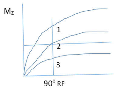
If you are asking why the Mz graph on the top does not go to zero at the vertical black line, that is simply because I did not update the upper graph or discuss what happens to Mz. The discussion was focused on the consequences for Mt and I had not bothered to update the upper graph. Apologies if this was confusing.
You are correct that in a properly designed spin echo pulse sequence, where sampling occurs at the moment 2*(TE/2), fat and water will be in phase. This is because the fat/water chemical shift IS a T2’ effect that may be compensated by the spin echo. To achieve out of phase images, the timing of TE would have to be altered. GRE is most widely used for Dixon imaging, but spin echo-based methods have also been created.
In multi-echo imaging AND in multi-slice imaging AND when multi-echo and multi-slice are combined, each TE contributes a single line of k-space to a single image per TR. In the following example:
Excite Slice #1 >> 180 >> TE-a >> 180 >> TE-b | Excite Slice #2 >> 180 >> TE-a >> 180 >> TE-b | …….TR Excite Slice #1….
The above is repeated at TR for the number of phase encoding steps required (Np)
We will generate a single line of data for the following 4 images:
Slice #1/TE-a
Slice #1/TE-b
Slice #2/TE-a
Slice #2/TE-b
Slices 1, 2 with TE-b will represent the same anatomy, at greater T2 contrast, compared to Slices 1 and 2 with TE-a.
The color scale reflects t-values in the image I displayed. It could reflect any statistic comparing the signal and stimulus paradigms.
1 and 3 would have almost equal signal, as it is the magnitude of the Mz which matters. Regardless of its orientation (up or down) Mz is rotated into the transverse plane, producing Mt, when the 90 RF is applied.